Wave Action on Piles
Calculate wave action forces on piles using Morison equation.
Wave Parameters
A progressive wave presents a period T, a wavelength Lw (distance from one crest to another), a height H (distance between trough and crest) and a form η. The figure below illustrates the characteristics of the progressive wave, and Equation (1) presents the expression to determine the wave form as a function of abscissa x and time t.
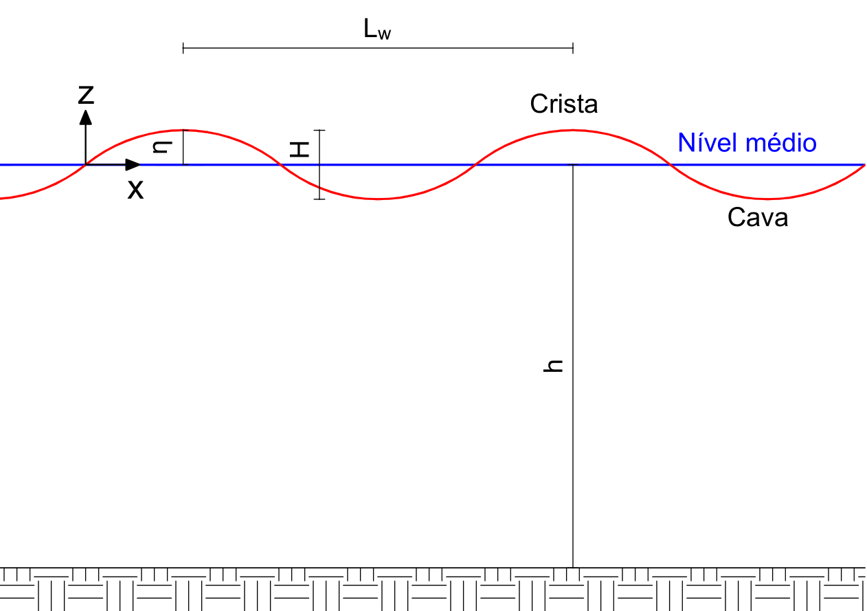
Figure 1: Schematic of progressive wave parameters.
(1)
Where σw is the angular frequency of the wave, and kw is the wave number:
(2)
(3)
Knowing the wave period T and the local depth h, the solution of the wave dispersion equation can provide the wavelength Lw. Therefore, the wave dispersion equation (4) is presented below, where g is the acceleration due to gravity.
(4)
Attempting to analytically solve Equation (4) for the wavelength results in Equation (5), which has no analytical solution. Its solution requires an iterative process of trials so that both sides of the equation converge to the same value.
(5)
The literature presents simplifications through boundary conditions to approximate the trigonometric function value present in the equation (hyperbolic tangent). These boundary conditions are checks regarding the wave propagation regime (shallow, intermediate, or deep waters). These simplifications are not addressed here. Once these parameters are known, it is possible to begin determining the forces caused by waves on structures.
Forces on Piles
To determine the forces exerted on a pile, Morison's formula is widely used in the literature, presented in standards such as the Spanish engineering standard (ROM 2.0-11) and the British standard (BS 6349-1-2), for use in the design of port or maritime structures.
Morison's Formula
Morison's equation addresses the forces caused on the pile through two terms. The first term of Equation (6) deals with the drag force from fluid motion. The second term deals with the effects of acceleration caused by wave motion. To fit experimentally obtained results, two coefficients are used, CD and CM. These are respectively drag and inertia coefficients (obtained experimentally), ρ is the specific mass of the water or fluid, Dp the pile diameter, and uw the horizontal component of particle velocity under the wave. Morison's formula is presented below:
(6)
The horizontal component of particle velocity during wave passage uw depends on the wave theory used. Linear theory is used here, so the equations describing this component and its time derivative follow below:
(7)
(8)
Substituting the respective components into Equation (6), it is possible to separate and treat the terms in isolation. Thus, after separation and algebraic manipulation, we have Equations (9) and (10) for drag and inertia forces per unit length, respectively.
(9)
(10)
To obtain the maximum effort caused by the drag force, one can consider the maximum values for the cosine terms, i.e., when t is zero, at which point the wave crest is in contact with the pile. This yields Equation (11).
(11)
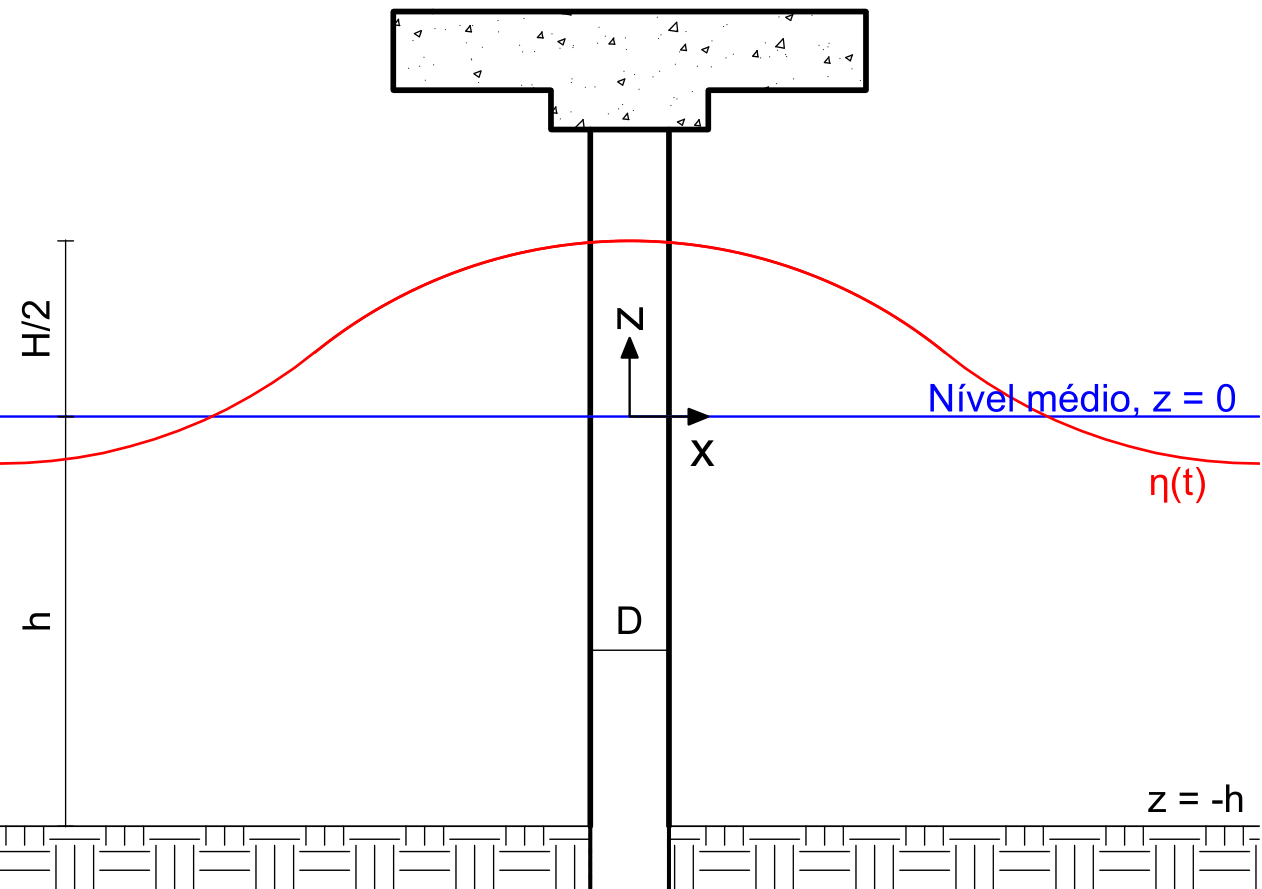
Figure 2: Schematic for maximum drag effort.
To obtain the maximum effort caused by the inertia force, one can consider the maximum value for the sine term, i.e., when t is negative at one quarter of the wave period (-T/4). This yields Equation (12).
(12)
To better illustrate the responses of FD and FM, Figure 3 presents the approximate profile of load distribution along the pile. The profile is similar for both components (neglecting wave form and position). In Figure 3 the pile diameter was omitted.
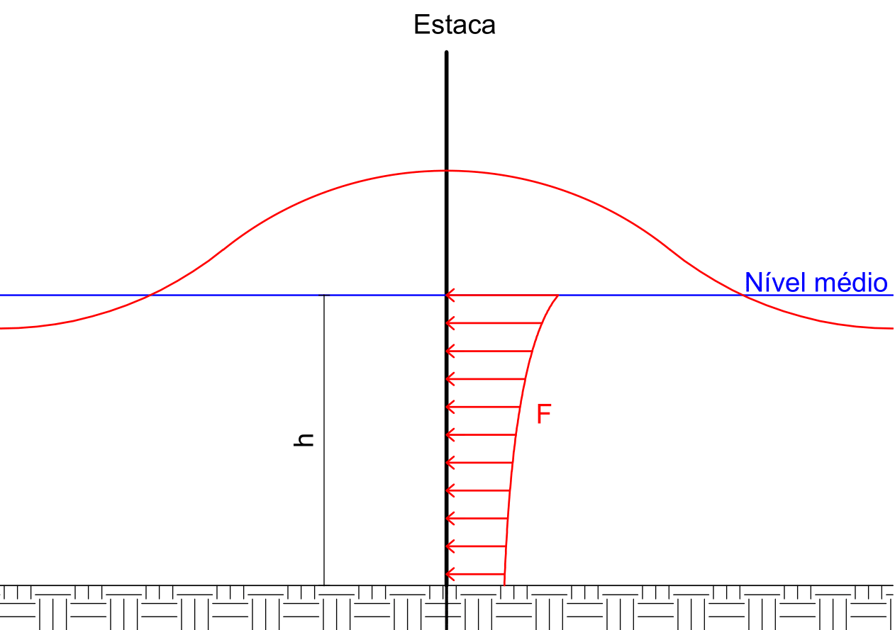
Figure 3: Schematic for load distribution profile on the pile.
Resultants
Since Equations (11) and (12) provide force per unit length of the pile, the resultant force can be obtained by integration. The method adopted by Mason and Dean neglects the wave surface, i.e., forces are calculated from the waterline down, these relations being valid for Dp/Lw < 0.05, something generally verified in engineering practice. Therefore, we have:
(13)
(14)
The application points of these forces, distant dD and dM from the base, are used for determining the acting moments, commonly applied during the design of these structures, and can be found approximately by expressions (15) and (16). Figure 4 shows a schematic of the resultant force and its application point.
(15)
(16)
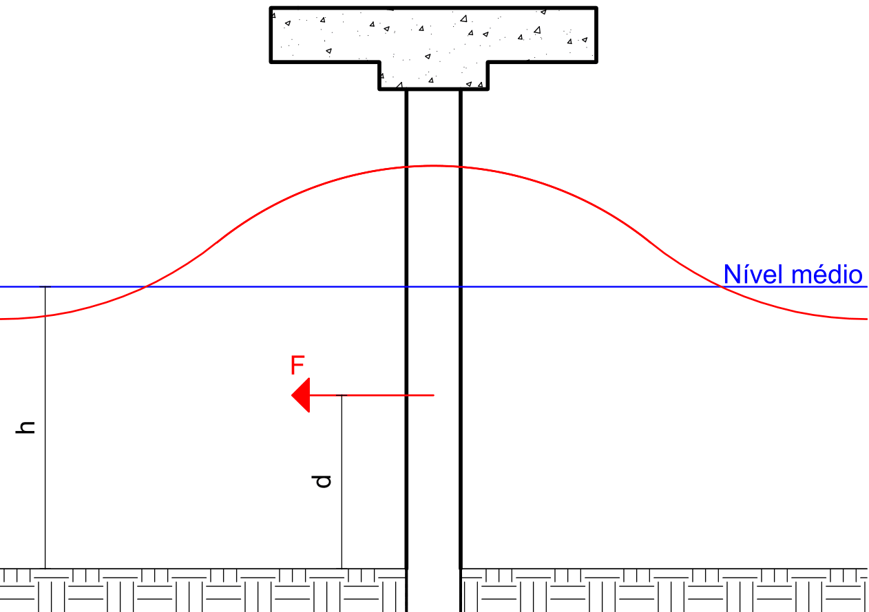
Figure 4: Schematic of resultant force and application point.
References
- BS 6349. Maritime works - Part 1-2: General — Code of practice for assessment of actions. [S.l.]: BSI Standards Limited, 2017. ISBN 9780580988318.
- MASON, J. Obras Portuárias. 1. ed. Rio de Janeiro, RJ: Editora Campus, 1981.
- MORISON, J. R.; JOHNSON, J. W.; SCHAAF, S. A. The Force Exerted by Surface Waves on Piles. Journal of Petroleum Technology, v. 2, n. 05, p. 149–154, 05 1950. ISSN 0149-2136. Disponível em: <https://doi.org/10.2118/950149-G>.
- ROM 2.0-11. Recomendaciones para el proyecto y ejecución en Obras de Atraque y Amarre. [S.l.]: Puertos del Estado, 2012. (Recomendaciones para Obras Marítimas. Serie 2, Obras portuárias interiores).